Biodiesel Supply Response to Production Profits

In a post last week the profitability of biodiesel production was examined. The analysis found that since the beginning of 2013 diesel blenders had bid up the price of biodiesel substantially in relation to the price of soybean oil, the main feedstock used to make biodiesel in the U.S. This drove biodiesel production profits to levels rarely seen in recent years. It was argued that there were likely two explanations for the spike in profits: i) diesel blenders were motivated to incentivize an increase in the production of biodiesel during 2013 to take advantage of the blenders tax credit that was reinstated only for this year; and ii) the biodiesel mandate under the RFS was expanded by the EPA from 1 billion gallons in 2012 to 1.28 billion gallons in 2013 and there may be a need for additional production above the mandate in 2013 in order to meet parts of the advanced and renewable mandates. Here, the analysis is extended to examine the impact of the rising profits on the quantity of biodiesel produced.

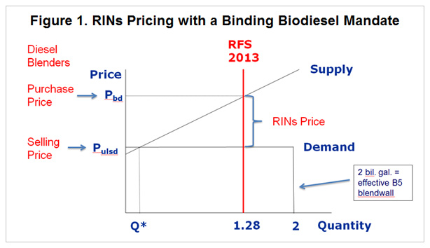
The responsiveness of biodiesel supply to profits plays a key role in determining the price of D4 biodiesel and D6 ethanol RINs (see the posts here and here for detailed explanations). Given the controversy that has erupted about potential manipulation in the RINs market, understanding the dynamics of biodiesel supply is more important than ever. We start with a conceptual analysis of the impact of biodiesel supply on RINs pricing, as illustrated in Figure 1. The model includes two important changes relative to the supply and demand curves for biodiesel used in previous posts. First, demand is perfectly elastic (horizontal) for biodiesel prices equal to ultra low sulfur diesel prices up to the technical limit on use. This reflects an assumption that biodiesel and ultra low sulfur diesel are perfect substitutes. Put another way, the breakeven price for biodiesel blending is assumed to be the price of diesel. Second, demand becomes perfectly inelastic (vertical) at an assumed B5 blendwall of 2 billion gallons. This technical limitation was highlighted in the EPA’s RFS rulemaking for 2013 (see p. 49815). According to the EPA, diesel engines were not warrantied for biodiesel blends above 5 percent previous to 2011. Newer engines are warrantied for higher blends but the EPA did not have access to the proportion this represents of the total fleet of diesel vehicles. With diesel consumption of 50 billion gallons, the computed B5 blendwall is 2.5 billion gallons (0.05 X 50). We follow the EPA and use an effective B5 blendwall of 2 billion gallons to account for lower biodiesel blends used in cold climates during the winter due to gelling issues. Finally, note that we do not account for the blenders tax credit in Figure 1 in order to simplify the presentation. We will have more to say about this later in the post.

Figure 1 implies that the 2013 RFS mandate of 1.28 billion gallons is highly binding. That is, the mandated quantity far exceeds the small amount of biodiesel that would be produced in the U.S. absent the RFS mandate (Q*). In order to get the higher than equilibrium quantity produced, biodiesel producers must be paid a price that is higher (Pbd) than the breakeven diesel price (Pulsd). From the perspective of a diesel blender, there is a wedge between the price they pay biodiesel producers and the price they charge consumers for the biodiesel in diesel blends. This wedge, or loss, is exactly equal to the price of a D4 biodiesel RIN. One can easily see that the D4 RIN price will therefore vary directly with the steepness (slope) and position (intercept) of the biodiesel supply curve.

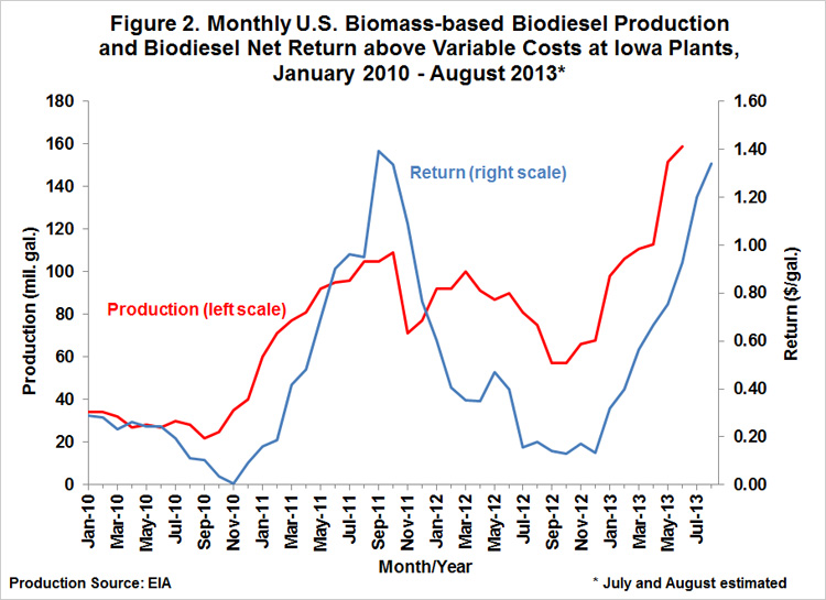
With that background, we now turn to the task of estimating the responsiveness of biodiesel production to profitability. Figure 2 presents a time-series plot of monthly biodiesel production estimated by the EIA and monthly biodiesel production net returns above variable costs over January 2010-August 2013. Returns are based on the model of a representative Iowa biodiesel plant first presented in this post from last week. Monthly profits are computed as the average of the weekly profits. Returns above variable costs are examined since fixed costs are not relevant for short-run production decisions. Also note that July and August 2013 biodiesel production are estimated based on data from the EPA EMTS system, which does not have as long of reporting lag compared to the EIA system. The figure shows tremendous variability in production and returns. Both peaked in late-2011 and again in mid-2013. Troughs were observed in late-2010 and late-2012. The timing of the peaks and troughs is not accidental. The blenders tax credit was not in place for 2010, was restored in 2011, lapsed again in 2012, and then was restored again for 2013. Despite this changing policy environment Figure 2 clearly shows that biodiesel production could be quite responsive to net returns.

A more detailed view of production responsiveness is shown in Figure 3. Following the analysis found in a May 2013 CARD report from Iowa State University, the scatter of monthly production and returns is plotted for each calendar year separately. This is done because in years when the blenders tax credit is not in place there is little relationship between biodiesel production and returns. The reason can be seen by referring back to Figure 1. Basically, production in this scenario is “stuck” at the mandate regardless of the level of returns (more technically, shifts in supply and demand curves do not change market quantities over a wide range of outcomes). The flat fitted regression lines for 2010 and 2012 in Figure 3 confirm this observation. One has to be careful to avoid the mistake of arguing that when the tax credit is restored a more normal upward sloping response curve will be observed. If market participants expect the credit to be in place permanently then market prices will adjust but production will remain stuck at the mandate. However, if market participants expect the credit to expire at the end of a calendar year then there is an obvious incentive for blenders to bid up the price of biodiesel in order to increase production and take full advantage of the credit before it expires. This appears to be exactly what happened in 2011 and is currently happening in 2013. In essence, these unique market circumstances provide an opportunity to learn something about the responsiveness of biodiesel production to profitability even though a seemingly binding RFS mandate is in place.

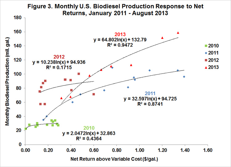
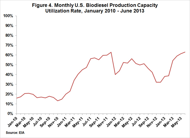
It is interesting to observe in Figure 3 that the production response in 2013 is much larger than in 2011 for the same level of net returns. It is not completely clear why this is the case. One possibility is that biodiesel firms are more optimistic now about the longer-term outlook than in 2011 and are therefore more willing to invest in expanded production for a given level of returns. Regardless, both 2011 and 2013 provide interesting evidence on production responsiveness. The elasticity of monthly supply response evaluated at the 2013 mandate level of 1.28 billion gallons (106.667 million gallons per month) is 0.31 using the 2011 fitted regression and 0.61 using the 2013 fitted regression. In other words, a 1 percent increase in net returns above variable costs leads to a 0.31 percent increase in monthly production using the 2011 data and a 0.61 percent increase using 2013 data. These estimates seem quite reasonable, particularly in light of the large excess capacity that has characterized the U.S. biodiesel industry in recent years. Figure 4 shows that capacity utilization has been less than 20 percent at times and no more than about 60 percent, indicating there has been plenty of slack capacity to draw upon when profit opportunities are present.

Implications

Biodiesel production is quite responsive to profitability given the right market circumstances. This is one of the reasons why D4 and D6 RINs prices have not risen to even more elevated levels than already seen in 2013. The next challenge is to determine whether a supply curve based on the estimated relationships in combination with a demand curve can replicate the prices of D4 RINs actually traded in the marketplace. This will help answer some of the important questions that have been raised about the efficiency of price discovery in the RINs market