Revisiting the Estimation of Biomass-Based Diesel Supply Curves

Biomass-based diesel, which includes both biodiesel and renewable diesel, plays a critical role in compliance with RFS mandates. Since 2013, biomass-based diesel (BBD) has been the “marginal gallon” for complying not only with the advanced mandate but also the conventional (ethanol) mandate due to the constraints on ethanol consumption presented by the E10 blend wall. In the farmdoc daily article of July 19, 2017 we estimated the amount of BBD required to fill the BBD mandate and also fill the advanced and conventional gaps would be near three billion gallons in both 2017 and 2018. The bottom-line is that the responsiveness of BBD supply to price is central to determining the cost of complying with the RFS. In a related fashion, the price responsiveness of BBD supply plays a key role in determining the price of D4 biodiesel and D6 ethanol RINs, the tradeable credits used by obligated parties to demonstrate RFS compliance. Several previous farmdoc daily articles (e.g., October 17, 2013) include efforts to estimate the crucial BBD supply curves. In this article, we revisit the estimation of BBD supply curves with two notable improvements. First, we estimate the relationship between BBD quantity supplied and price directly. Second, we estimate supply curves for both domestically produced and imported BBD.

Conceptual Background

One can plot price and quantity for any commodity and draw a line through the observations. The problem is knowing what the relationship means, if anything. This is what economists call the “identification” problem (see Tomek and Kaiser, 2014, Ch. 14). Figure 1 provides a conceptual model of the BBD market that can be used to illustrate the challenge. The model in Figure 1 is the same conceptual model we have used in a number of earlier articles on biodiesel, the RFS, and RINs pricing (e.g., farmdoc daily, April 5, 2017). The model represents the supply of BBD producers and demand from diesel blenders at the wholesale level in a competitive market. Retail demand at the consumer level is implicitly represented by a simple percentage markup of the wholesale demand shown in Figure 1. This implies full pass through of wholesale price changes to the retail level. The model assumes an L-shaped demand curve, with the vertical perfectly inelastic portion equal to the fixed RFS volume mandate and the horizontal perfectly elastic portion above the mandate equal to ultra low sulfur diesel prices. This reflects an assumption that BBD and petroleum diesel are perfect substitutes (after adjustment for the lower energy value of most BBD) and that BBD is a small enough part of the diesel market that changes in the BBD price do not impact the overall demand for diesel fuel. As usual, equilibrium is found where the supply and demand curves intersect.

Figure 2 illustrates a scenario where the demand curve is fixed and the supply curve shifts due to increasing and decreasing soybean oil prices. Since over 80 percent of the production cost of BBD is feedstock costs, the main factor shifting the supply curve in this model is soybean oil prices. Due to the binding nature of the RFS volume mandate, the shifts in supply simply move the BBD price up and down without changing the equilibrium quantity. In this situation, it is impossible to identify the supply curve based on the equilibrium price and quantity observations. Figure 3 illustrates just the opposite scenario where the supply curve is fixed and the demand curve changes due to changes in the RFS volume mandate (but fixes the price of petroleum diesel). Now the equilibrium price and quantity observations exactly trace out the supply curve and allow perfect identification.

It is not unusual in practice for supply and demand curves to both shift at the same time. Commodity markets are highly dynamic and BBD is no exception. Figure 4 illustrates the scenario where the shifts in supply and demand are roughly of the same magnitude. This results in a “shotgun” scatter of observed price and quantity observations that allows only a poor identification (tracing out) of the underlying supply curve. In contrast, Figure 5 shows a scenario where the demand shifts are much larger than the supply shifts, which allows a strong identification of the supply curve based on observed prices and quantities. In essence, the demand shifts due to the changing volume mandates are larger than the supply shifts due to changing soybean oil prices and this is the key to tracing out the underlying supply curve. This is the desired scenario for estimating BBD supply curves from actual market data. Lastly, it is importance to recognize that this type of identification is not perfect; rather, the average relationship between BBD quantity supplied and price is estimated.

Supply Curve Estimates

The analysis in the previous section provides a clear guide to identifying and estimating BBD supply curves. One needs to find periods where shifts in the demand curve are substantially larger than shifts in the supply curve. In the short-run (e.g., monthly or quarterly) this is ordinarily impossible to achieve since RFS volume mandates are fixed on an annual basis. This situation is well-illustrated by Figure 2. Fortunately, a unique opportunity to identify and estimate BBD supply and price responses is provided in years when the blenders tax credit is expected to expire (2011, 2013, 2016). As discussed in several previous articles (e.g., farmdoc daily, March 1, 2017), it is rational for diesel blenders to increase their demand for BBD within the year in a race to take advantage of the credit before it expires. In essence, blenders purchase BBD at a discount in the current year, due to the tax credit, in order to meet mandates in later years. This has the effect of increasing the volume mandate and shifting the demand curve as shown in Figure 3. They key is whether this variation in demand is larger than the variation in supply due to changing soybean oil prices.

We took advantage of this unique opportunity for identifying and estimating BBD supply curves using 2013 data in the farmdoc daily articles of September, 25, 2013 and particularly October 17, 2013. Following the analysis found in a May 2013 CARD report from Iowa State University, a best-fit regression line was fit to a scatter of monthly biodiesel production (y-axis) and estimated net returns (x-axis) for January – October 2013, with the natural log (ln) of production used as the dependent variable. Next, the y- and x-axes were flipped and monthly quantities were converted to annual quantities by multiplying monthly quantities by 12. The final step in estimating the supply curves was to plot the curve in terms of biodiesel price instead of net returns on the y-axis. This was accomplished by adding back to net returns all variable costs, including soybean oil, natural gas, and methanol costs, and subtracting glycerin revenue. The estimated BBD supply curves have several interesting and useful characteristics in terms of slope, computed supply elasticities, and supply curve shifters. However, the estimation procedure is somewhat complicated, being that it is a cost-derived supply curve. A direct estimate of a supply curve based on actual price and quantity observations is more appealing.

Here, we use monthly supply and price observations in 2016 to estimate BBD supply curves. As noted above, 2016 was a year when the biodiesel tax credit expired. In the farmdoc daily article of July 19, 2017, it was reported that the annual BBD supply for calendar year 2016 exceeded the amount of BBD required to fill both the BBD mandate and the RFS gaps by 20 percent (461 million gallons). Market participants expected the blenders tax credit to expire at the end of the year and there was an obvious incentive for blenders to bid up the price of biodiesel in order to increase production and take full advantage of the credit before it expired. We used the same procedure to estimate monthly BBD supply for 2016 as we used in the July 19 article to estimate annual supply with one exception. We did not allocate D4 RINs error corrections across months in 2016 as we lacked any information on the seasonal pattern of these corrections. The size of the annual error correction is very small so this should not bias the monthly estimates in a meaningful fashion.

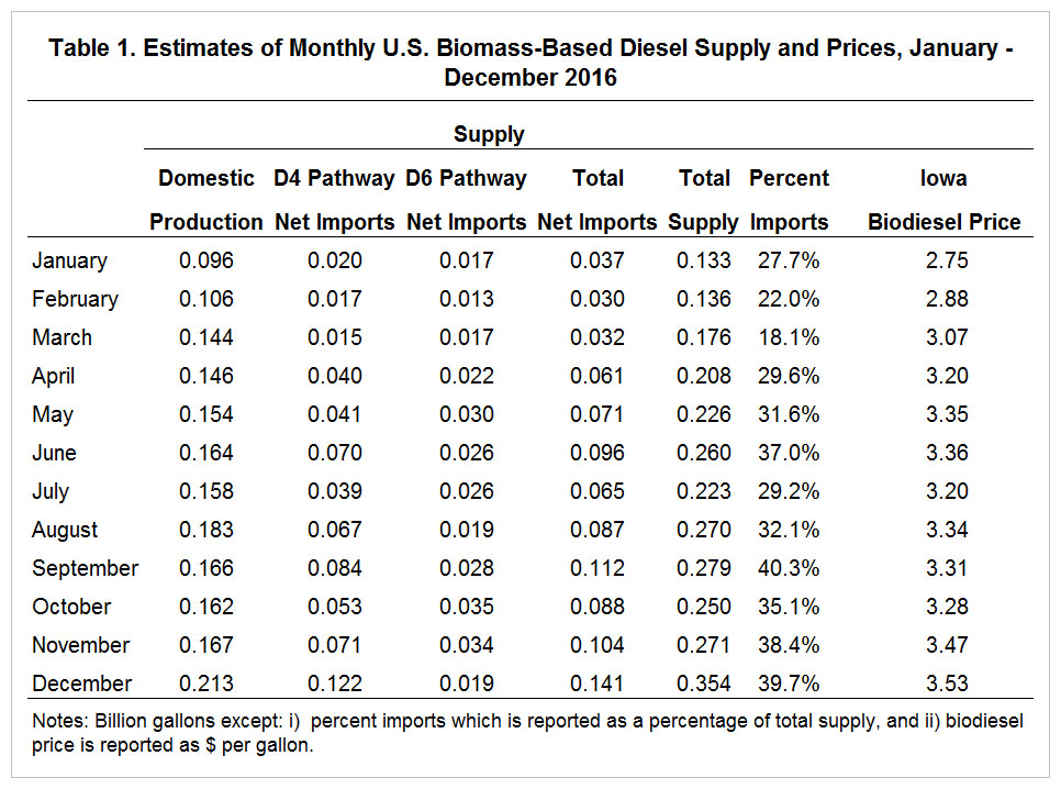
The monthly supply and biodiesel price data for 2016 are presented in Table 1. Supply estimates are made for five categories–domestic production, D4 pathway net imports, D6 pathway net imports, total net imports, and total supply. The Iowa biodiesel price is used to represent all BBD prices. Monthly supplies were in a surprisingly large range for all categories. For example, monthly domestic supply ranged from 96 to 213 million gallons and monthly total net imports ranged from 30 to 141 million gallons. The coefficient of variation (standard deviation divided by mean) is a standardized measure of variability that can be used for comparison across series that differ widely in their average levels. The coefficient of variation for the supply variables ranged from 20 percent for domestic production to 59 percent for D4 pathway imports. By comparison, the coefficient of variation for monthly biodiesel prices was only 7.1 percent. This suggests variability of supply shifts due to changing soybean oil prices was substantially less than the tax-credit induced changes in demand. There was some change in the price of soybean oil during the year. The price of soybean oil averaged $0.32 per pound for the year and was in a very narrow range during the first three quarters, before increasing during the final quarter. The average monthly price ranged from about $0.29 to about $0.37 per pound.

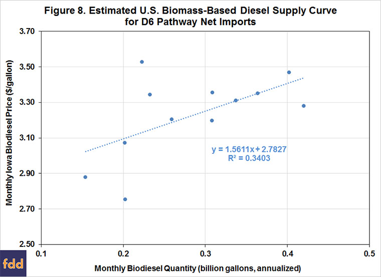
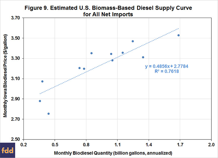
The monthly quantities shown in Table 1 are annualized by multiplying by 12 and the scatter of annualized quantities and monthly average prices of biodiesel are plotted for each of the five categories in Figures 6 through 10. A linear regression is then fit to the scatter of observations as an estimate of the supply curve for each category. The fit of the linear regressions to the price/quantity scatters is reasonably good except for D6 pathway net imports. For example, the R2 for the domestic and total supply curves is 0.8635 and 0.865, respectively. Given that the fit is reasonably good in four of the five categories, we can conclude that our strategy for identifying BBD supply curves worked well, especially when one considers that the samples only contain 12 observations. We can also infer that the variability of supply shifts due to changing soybean oil prices in 2016 was indeed substantially less than the tax-credit induced variability in demand. So, fortuitously, the data from 2016 most resemble Figure 6 rather than Figure 5.

The estimated supply curves have a very interesting characteristic that can be seen in the flexibilities and elasticities presented in Table 2. The flexibilities give the percentage change in price for a one-percentage point change in quantity supplied, while the elasticities give the percentage change in quantity supplied for a one-percentage point change in price. Both are evaluated at the average quantity for each category and the average biodiesel price. The price flexibilities are very low, implying that large price increases are not needed to elicit a large quantity response. For example, the domestic supply flexibility indicates that a one-percentage point increase in quantity supplied only requires a 0.33 percentage point increase in price. The supply elasticities are computed as the inverse of flexibilities and are all extremely large given the small flexibilities. This implies that a small price increase results in a huge increase in quantity supplied. For example, the supply elasticity for D4 pathway net imports is 10.19, which indicates that a one-percentage point increase in price results in a 10.19 percentage point increase in quantity. In economic terms, this means all of the estimated supply curves are extremely elastic. This is not surprising in light of the overbuilt nature of BBD production capacity both in the U.S. and overseas. As an example, domestic capacity utilization in the U.S. has only occasionally been higher than 65 percent (farmdoc daily, February 11, 2016). In this situation, prices do not have to cover the variable and fixed costs of production for slack capacity to be brought online; but, instead only have to cover variable costs because the capacity is already in place. This excess capacity presents a constant threat of over-production once BDD prices exceed variable costs of production.

Implications

Biomass-based diesel (BBD) supply curves represent a fundamental building block for analyzing RFS mandates because BBD has served as the “marginal” gallon for filling gaps in both the advanced and conventional mandates. We take advantage of the unique opportunity for identifying and estimating BBD supply curves that occurred in 2016 due to the expiration of the biodiesel tax credit. The fit of the estimated supply curves is reasonably good except for D6 pathway net imports. For example, the R2 for the domestic and total supply curves is 0.8635 and 0.865, respectively. The estimated supply curves have the interesting characteristic of being extremely elastic. As one example, the supply elasticity for D4 pathway net imports is 10.19, which indicates that a one-percentage point increase in price results in a 10.19 percentage point increase in quantity.

The estimated supply curves will be used in future farmdoc daily articles to analyze several issues, including the potential price impact of expanding total BBD supply requirements and policy changes that could require much larger domestic supplies. One issue is that supply requirements could be influenced by the outcome of litigation challenging the EPA’s ‘inadequate domestic supply”‘ argument that limited the conventional ethanol mandate relative to the statutory mandate in 2014, 2015, and 2016. A requirement to backfill that shortfall would likely require larger quantities of BBD. In addition to total BBD supply, the source of supply (domestic or imported) could also become an issue. For example, changes in domestic biodiesel policy and/or WTO rulings could dramatically reduce BBD imports, in effect making the U.S. a BBD island. Specifically, a change from a blender to a domestic producer tax credit (assuming the tax credit is reinstated) would essentially shut out imports of BBD to the U.S. Similarly, a World Trade Organization (WTO) finding of unfair BBD trade practices by Indonesia and Argentina would reduce or eliminate imports from two important sources. Expanding BBD supply requirements and increasing dependence on domestic BBD production could have important implications for the price of BBD.

References

Babcock, B., M. Moreira, and Y. Peng. "Biofuel Taxes, Subsidies, and Mandates: Impacts on Us and Brazilian Markets." Staff Report 13-SR 108, Center for Agricultural and Rural Development, Iowa State University, May 22, 2013. http://www.card.iastate.edu/products/publications/pdf/13sr108.pdf
Irwin, S and D. Good. "Filling the Gaps in the Renewable Fuels Standard with Biodiesel." farmdoc daily (7):130, Department of Agricultural and Consumer Economics, University of Illinois at Urbana-Champaign, July 19, 2017.
Irwin, S. "Blender and Producer Sharing of Retroactively Reinstated Biodiesel Tax Credits: Time for a Change?" farmdoc daily (7):62, Department of Agricultural and Consumer Economics, University of Illinois at Urbana-Champaign, April 5, 2017.
Irwin, S. "The Profitability of Biodiesel Production in 2016." farmdoc daily (7):38, Department of Agricultural and Consumer Economics, University of Illinois at Urbana-Champaign, March 1, 2017.
Irwin, S. "The Profitability of Biodiesel Production in 2015." farmdoc daily (6):27, Department of Agricultural and Consumer Economics, University of Illinois at Urbana-Champaign, February 11, 2016.
Irwin, S. "Estimating the Biomass-Based Diesel Supply Curve." farmdoc daily (3):237, Department of Agricultural and Consumer Economics, University of Illinois at Urbana-Champaign, December 13, 2013.
Irwin, S. "Estimating the Biodiesel Supply Curve." farmdoc daily (3):198, Department of Agricultural and Consumer Economics, University of Illinois at Urbana-Champaign, October 17, 2013.
Irwin, S. "Biodiesel Supply Response to Production Profits." farmdoc daily (3):182, Department of Agricultural and Consumer Economics, University of Illinois at Urbana-Champaign, September 25, 2013.
Tomek, W.G., and H.M. Kaiser. Agricultural Product Prices, Fifth Edition. Cornell University Press: Ithaca, NY, 2014.
Disclaimer: We request all readers, electronic media and others follow our citation guidelines when re-posting articles from farmdoc daily. Guidelines are available here. The farmdoc daily website falls under University of Illinois copyright and intellectual property rights. For a detailed statement, please see the University of Illinois Copyright Information and Policies here.